Quantum Monte Carlo

1. Introduction

This website contains the QMC tutorial of the 2023 LTTC winter school Tutorials in Theoretical Chemistry.

We propose different exercises to understand quantum Monte Carlo (QMC) methods. In the first section, we start with the computation of the energy of a hydrogen atom using numerical integration. The goal of this section is to familiarize yourself with the concept of local energy. Then, we introduce the variational Monte Carlo (VMC) method which computes a statistical estimate of the expectation value of the energy associated with a given wave function, and apply this approach to the hydrogen atom. Finally, we present the diffusion Monte Carlo (DMC) method which we use here to estimate the exact energy of the hydrogen atom and of the H₂ molecule, starting from an approximate wave function.

Code examples will be given in Python3, C and Fortran. You can use whatever language you prefer to write the programs.

We consider the stationary solution of the Schrödinger equation, so the wave functions considered here are real: for an $N$ electron system where the electrons move in the 3-dimensional space, $Ψ : R^{3 N} \to R$ . In addition, $Ψ$ is defined everywhere, continuous, and infinitely differentiable.

All the quantities are expressed in atomic units (energies, coordinates, etc).

1.1. Energy and local energy

For a given system with Hamiltonian $\hat{H}$ and wave function $Ψ$ , we define the local energy as

$E_{L} (r) = \frac{\hat{H} Ψ (r)}{Ψ (r)},$

where $r$ denotes the 3N-dimensional electronic coordinates.

The electronic energy of a system, $E$ , can be rewritten in terms of the local energy $E_{L} (r)$ as

\begin{array}{rcl} E & = & \frac{⟨ Ψ | \hat{H} | Ψ ⟩}{⟨ Ψ | Ψ ⟩} = \frac{\int Ψ (r) \hat{H} Ψ (r) d r}{\int | Ψ (r) |^{2} d r} \\ = & \frac{\int | Ψ (r) |^{2} \frac{\hat{H} Ψ (r)}{Ψ (r)} d r}{\int | Ψ (r) |^{2} d r} = \frac{\int | Ψ (r) |^{2} E_{L} (r) d r}{\int | Ψ (r) |^{2} d r} \end{array}

For few dimensions, one can easily compute $E$ by evaluating the integrals on a grid but, for a high number of dimensions, one can resort to Monte Carlo techniques to compute $E$ .

To this aim, recall that the probabilistic expected value of an arbitrary function $f (x)$ with respect to a probability density function $P (x)$ is given by

$⟨ f ⟩_{P} = \int_{- \infty}^{\infty} f (x) P (x) d x$

where the probability density function $P (x)$ is non-negative and integrates to one:

$\int_{- \infty}^{\infty} P (x) d x = 1.$

Similarly, we can view the energy of a system, $E$ , as the expected value of the local energy with respect to a probability density $P (r)$ defined in $3 N$ dimensions:

$E = \int E_{L} (r) P (r) d r \equiv ⟨ E_{L} ⟩_{P},$

where the probability density is given by the square of the wave function:

$P (r) = \frac{| Ψ (r) |^{2}}{\int | Ψ (r) |^{2} d r} .$

If we can sample $N_{M C}$ configurations ${r}$ distributed as $P$ , we can estimate $E$ as the average of the local energy computed over these configurations:

$E \approx \frac{1}{N_{M C}} \sum_{i = 1}^{N_{M C}} E_{L} (r_{i}) .$

Here is an animation of the local energy in the N₂ molecule along a QMC trajectory:

Contents:

1.1. Energy and local energy

2. Numerical evaluation of the energy of the hydrogen atom

In this section, we consider the hydrogen atom with the following wave function:

$Ψ (r) = \exp (- a | r |)$

We will first verify that, for a particular value of $a$ , $Ψ$ is an eigenfunction of the Hamiltonian

$\hat{H} = \hat{T} + \hat{V} = - \frac{1}{2} Δ - \frac{1}{| r |}$

To do that, we will compute the local energy and check whether it is constant.

2.1. Local energy

You will now program all quantities needed to compute the local energy of the Hydrogen atom for the given wave function.

Write all the functions of this section in a single file : hydrogen.py if you use Python, hydrogen.F90 if you use Fortran, or hydrogen.c and hydrogen.h if you use C.

When computing a square root in $R$ , always make sure that the argument of the square root is non-negative.
When you divide, always make sure that you will not divide by zero

If a floating-point exception can occur, you should make a test to catch the error.

2.1.2. Exercise 1

Write a function called potential that takes a single argument r, which is an array of 3 double precision numbers. The function calculates the distance from the origin using the Euclidean distance formula, and then calculates the potential using this distance. If the distance is 0, the program prints a warning that the potential diverges. If the distance is greater than 0, the potential is calculated as

$V (r) = - \frac{1}{\sqrt{x^{2} + y^{2} + z^{2}}}, with r = (\begin{matrix} x \\ y \\ z \end{matrix}),$

Python

#!/usr/bin/env python3
import numpy as np

def potential(r):
    # TODO

def test_potential():
    expected_output = -1./15.
    for r in [( 2., 5., 14.), (5., 14., 2.), 
              (-2., 5.,-14.), (5.,-14.,-2.), 
              ( 0., 9.,-12.), (9.,-12., 0.)]:
          assert potential(r) == expected_output

    r = (0., 0., 0.)
    assert potential(r) == -float("inf")

    print("potential ok")

if __name__ == "__main__":
    test_potential()

Fortran

If the extension of your file is .F90 and not .f90, the C preprocessor will be called before compiling. This enables the possibility to have conditional compilation with #ifdef statements, activated with the -D compiler option.

To compile your code and activate the test, use:

gfortran -DTEST_H hydrogen.F90 -o test_hydrogen

double precision function potential(r)
  implicit none
  double precision, intent(in) :: r(3)

  ! TODO

end function potential

subroutine test_potential
    implicit none
    double precision :: r(3)
    double precision :: expected_output
    double precision, external :: potential

    expected_output = -1.d0/15.d0

    r(:) = (/ 2.d0, 5.d0, 14.d0 /)
    if (potential(r) /= expected_output) stop 'Failed'

    r(:) = (/ 5.d0, 14.d0, 2.d0 /)
    if (potential(r) /= expected_output) stop 'Failed'

    r(:) = (/ -2.d0, 5.d0, -14.d0 /)
    if (potential(r) /= expected_output) stop 'Failed'

    r(:) = (/ 5.d0, -14.d0, -2.d0 /)
    if (potential(r) /= expected_output) stop 'Failed'

    r(:) = (/ 0.d0, 9.d0, 12.d0 /)
    if (potential(r) /= expected_output) stop 'Failed'

    r(:) = (/ 9.d0, -12.d0, 0.d0 /)
    if (potential(r) /= expected_output) stop 'Failed'

    r(:) = 0.d0
    expected_output = -huge(1.d0)
    if (potential(r) /= expected_output) stop 'Failed r=0'
    print *, 'potential ok'

end subroutine test_potential

#ifdef TEST_H
program test_h
  call test_potential
end program test_h
#endif

Compile your code with the -DTEST_H option. It will activate the creation of the main function that will test your functions. Don't forget to use -lm to link with the math library.

gcc -DTEST_H hydrogen.c -lm -o test_hydrogen

#include <stdio.h>   // printf
#include <math.h>    // sqrt
#include <stdlib.h>  // exit
#include <assert.h>  // assert

double potential(double r[3]) {
  // TODO
}

static void test_potential() {
    double r[3];
    double expected_output;

    expected_output = -1./15.;
    r[0] = 2.;   r[1] =  5.;   r[2] = 14.;
    assert (potential(r) == expected_output);

    r[0] = 5.;   r[1] = 14.;   r[2] = 2.;
    assert (potential(r) == expected_output);

    r[0] = -2.;   r[1] = 5.;   r[2] = -14.;
    assert (potential(r) == expected_output);

    r[0] = 5.;   r[1] = -14.;   r[2] = -2.;
    assert (potential(r) == expected_output);

    r[0] = 0.;   r[1] = 9.;   r[2] = 12.;
    assert (potential(r) == expected_output);

    r[0] = 9.;   r[1] = -12.;   r[2] = 0.;
    assert (potential(r) == expected_output);

    expected_output = -HUGE_VAL;
    r[0] = 0.;   r[1] = 0.;   r[2] = 0.;
    assert (potential(r) == expected_output);

    printf("potential ok\n");
}

#ifdef TEST_H
int main() {
    test_potential();
    return 0;
}
#endif

2.1.3. Exercise 2

Write a function called psi that takes two arguments: a which is a double precision number, and r which is an array of 3 double precision numbers. The function calculates and returns the value of the wave function at the given point $r$ .

Python
```
def psi(a, r):
    # TODO
```

Fortran

double precision function psi(a, r)
  implicit none
  double precision, intent(in) :: a, r(3)

  ! TODO

end function psi

double psi(double a, double r[3]) {
  // TODO
}

2.1.4. Exercise 3

Write a function called kinetic that takes two arguments: a which is a double precision number, and r which is an array of 3 double precision numbers. The function calculates the local kinetic energy at the given point $r$ .

It first calculates the distance from the origin using the Euclidean distance formula. If the distance is greater than 0, the kinetic energy is calculated using the formula given below. If the distance is 0, the program prints a warning.

The local kinetic energy is defined as $T_{L} (r) = - \frac{1}{2} \frac{Δ Ψ (r)}{Ψ (r)} .$

We differentiate $Ψ$ with respect to $x$ :

$Ψ (r) = \exp (- a | r |)$ $\frac{\partial Ψ}{\partial x} = \frac{\partial Ψ}{\partial | r |} \frac{\partial | r |}{\partial x} = - \frac{a x}{| r |} Ψ (r)$

and we differentiate a second time:

$\frac{\partial^{2} Ψ}{\partial x^{2}} = (\frac{a^{2} x^{2}}{| r |^{2}} - \frac{a (y^{2} + z^{2})}{| r |^{3}}) Ψ (r) .$

The Laplacian operator $Δ = \frac{\partial^{2}}{\partial x^{2}} + \frac{\partial^{2}}{\partial y^{2}} + \frac{\partial^{2}}{\partial z^{2}}$ applied to the wave function gives:

$Δ Ψ (r) = (a^{2} - \frac{2 a}{| r |}) Ψ (r) .$

Therefore, the local kinetic energy is $T_{L} (r) = - \frac{1}{2} (a^{2} - \frac{2 a}{| r |})$

Python
```
def kinetic(a,r):
    # TODO
```

Fortran

double precision function kinetic(a,r)
  implicit none
  double precision, intent(in) :: a, r(3)

  ! TODO

end function kinetic

double kinetic(double a, double r[3]) {
  //TODO
}

2.1.5. Exercise 4

Write a function called e_loc that takes two arguments: a which is a double precision number and r which is an array of 3 double precision numbers. The function calculates the local energy at the given point $r$ .

It uses two functions kinetic and potential to calculate the kinetic energy and potential energy respectively and add them to get the local energy.

$E_{L} (r) = - \frac{1}{2} \frac{Δ Ψ}{Ψ} (r) + V (r)$

Python
```
def e_loc(a,r):
    #TODO
```
Fortran
When you call a function in Fortran, you need to declare its return type. You might by accident choose a function name which is the same as an internal function of Fortran. So it is recommended to always use the keyword external to make sure the function you are calling is yours.
```
double precision function e_loc(a,r)
  implicit none
  double precision, intent(in) :: a, r(3)

  double precision, external :: kinetic
  double precision, external :: potential

  ! TODO

end function e_loc
```

double e_loc(double a, double r[3]) {
  // TODO
}

2.1.6. Exercise 5

Find the theoretical value of $a$ for which $Ψ$ is an eigenfunction of $\hat{H}$ .

Contents:

2.2. Plot of the local energy along the $x$ axis

The program you will write in this section will be written in another file (plot_hydrogen.py, plot_hydrogen.F90 or plot_hydrogen.c for example). It will use the functions previously defined. If you use C, don't forget to write the header file corresponding to the functions defined in the previous section.

In Python, you should put at the beginning of the file

#!/usr/bin/env python3

from hydrogen import e_loc

to be able to use the e_loc function of the hydrogen.py file.

It is better to use #!/usr/bin/env python3 than #!/usr/bin/python because:

you are sure you are not using Python2, which is incompatible with Python3 syntax,
if you are on a machine where you can load different environments (VirtualEnv, module, etc), you will use the python3 provided by your environment, and not the system's one.

In Fortran, you will need to compile all the source files together:

gfortran hydrogen.F90 plot_hydrogen.F90 -o plot_hydrogen

Similarly, in C

gcc hydrogen.c plot_hydrogen.c -lm -o plot_hydrogen

In C, you need the -lm argument to link with the math library that contains functions like sqrt and exp.

2.2.1. Exercise

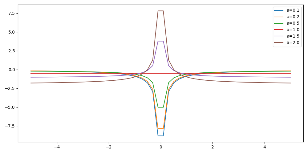
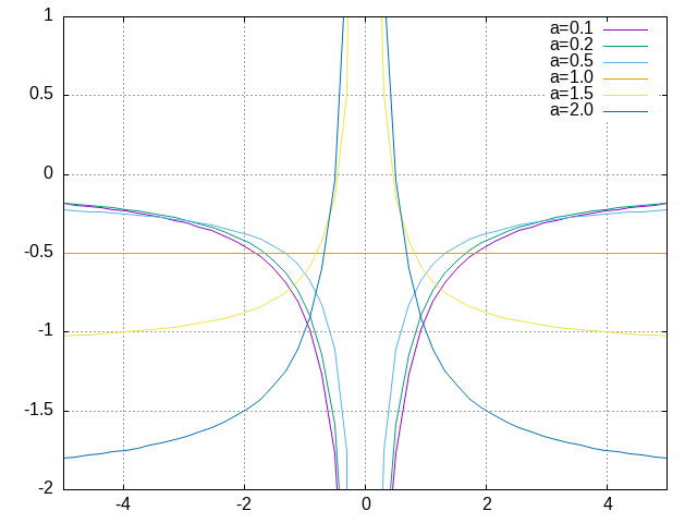
For multiple values of $a$ (0.1, 0.2, 0.5, 1., 1.5, 2.), plot the local energy along the $x$ axis.

In Python, you can use matplotlib for example.

In Fortran, it is convenient to write in a text file the values of $x$ and $E_{L} (r)$ for each point, and use Gnuplot to plot the files. With Gnuplot, you will need 2 blank lines to separate the data corresponding to different values of $a$ :

The potential and the kinetic energy both diverge at $r = 0$ , so we choose a grid that doesn't contain the origin to avoid numerical issues.

Python

#!/usr/bin/env python3

import numpy as np
import matplotlib.pyplot as plt

from hydrogen import e_loc

x=np.linspace(-5,5)
plt.figure(figsize=(10,5))

# TODO

plt.tight_layout()
plt.legend()
plt.savefig("plot_py.png")

Fortran

program plot
  implicit none
  double precision, external :: e_loc

  double precision :: x(50), dx
  integer :: i, j

  dx = 10.d0/(size(x)-1)
  do i=1,size(x)
     x(i) = -5.d0 + (i-1)*dx
  end do

  ! TODO

end program plot

To compile and run:

gfortran hydrogen.F90 plot_hydrogen.F90 -o plot_hydrogen
./plot_hydrogen > data

#include <stdio.h>
#include <math.h>
#include "hydrogen.h"

#define NPOINTS  50
#define NEXPO     6

int main() {

    double x[NPOINTS], energy, dx, r[3];
    double a[NEXPO] = { 0.1, 0.2, 0.5, 1.0, 1.5, 2.0 };
    int i, j;

    dx = 10.0/(NPOINTS-1);
    for (i = 0; i < NPOINTS; i++) {
        x[i] = -5.0 + i*dx;
    }

    // TODO
    return 0;
}

To compile and run:

gcc hydrogen.c plot_hydrogen.c -lm -o plot_hydrogen
./plot_hydrogen > data

Plotting for Fortran of C

Plot the data using Gnuplot:

set grid
set xrange [-5:5]
set yrange [-2:1]
plot './data' index 0 using 1:2 with lines title 'a=0.1', \
     './data' index 1 using 1:2 with lines title 'a=0.2', \
     './data' index 2 using 1:2 with lines title 'a=0.5', \
     './data' index 3 using 1:2 with lines title 'a=1.0', \
     './data' index 4 using 1:2 with lines title 'a=1.5', \
     './data' index 5 using 1:2 with lines title 'a=2.0'

Contents:

2.2.1. Exercise

2.3. Numerical estimation of the energy

If the space is discretized in small volume elements $r_{i}$ of size $δ r$ , the expression of $⟨ E_{L} ⟩_{Ψ^{2}}$ becomes a weighted average of the local energy, where the weights are the values of the square of the wave function at $r_{i}$ multiplied by the volume element:

$⟨ E ⟩_{Ψ^{2}} \approx \frac{\sum_{i} w_{i} E_{L} (r_{i})}{\sum_{i} w_{i}}, w_{i} = {| Ψ (r_{i}) |}^{2} δ r$

The energy is biased because:

The volume elements are not infinitely small (discretization error)
The energy is evaluated only inside the box (incompleteness of the space)

2.3.1. Exercise

Compute a numerical estimate of the energy using a grid of $50 \times 50 \times 50$ points in the range $(- 5, - 5, - 5) \leq r \leq (5, 5, 5)$ .

Python

#!/usr/bin/env python3

import numpy as np
from hydrogen import e_loc, psi

interval = np.linspace(-5,5,num=50)
delta = (interval[1]-interval[0])**3

r = np.array([0.,0.,0.])

for a in [0.1, 0.2, 0.5, 0.9, 1., 1.5, 2.]:
    # TODO
    print(f"a = {a} \t E = {E}")

Fortran

program energy_hydrogen
  implicit none
  double precision, external :: e_loc, psi
  double precision :: x(50), w, delta, energy, dx, r(3), a(6), normalization
  integer :: i, k, l, j

  a = (/ 0.1d0, 0.2d0, 0.5d0, 1.d0, 1.5d0, 2.d0 /)

  dx = 10.d0/(size(x)-1)
  do i=1,size(x)
     x(i) = -5.d0 + (i-1)*dx
  end do

  do j=1,size(a)

     ! TODO

     print *, 'a = ', a(j), '    E = ', energy
  end do

end program energy_hydrogen

To compile the Fortran code and run it:

gfortran hydrogen.F90 energy_hydrogen.F90 -o energy_hydrogen
./energy_hydrogen

C
```
#include <stdio.h>
#include <math.h>
#include "hydrogen.h"

#define NPOINTS  50
#define NEXPO     6

int main() {

    double x[NPOINTS], energy, dx, r[3], delta, normalization, w;
    double a[NEXPO] = { 0.1, 0.2, 0.5, 1.0, 1.5, 2.0 };

    dx = 10.0/(NPOINTS-1);
    for (int i = 0; i < NPOINTS; i++) {
        x[i] = -5.0 + i*dx;
    }

    for (int j = 0; j < NEXPO; j++) {
        // TODO
        printf("a = %f    E = %f\n", a[j], energy);
    }
}
```
To compile the C code and run it:
```
gcc hydrogen.c energy_hydrogen.c -lm -o energy_hydrogen
./energy_hydrogen 
```
Hints if you are stuck

The program starts by defining some variables and arrays, including an array a that contains 6 different values of the parameter a which will be used in the e_loc and psi functions to calculate the local energy and wave function respectively.

The program then calculates the value of dx, which is the step size in $x$ , and sets up an array x that contains 50 equally spaced points between -5 and 5. The program sets all elements of the r array to 0, and then enters a nested loop structure. The outer loop iterates over the values of a in the a array, and the next three loops iterate over the values of x in the x array for the three dimensions. For each value of a and x, the program sets the first element of the r array to the current value of x, calls the psi function to calculate the wave function, calls the e_loc function to calculate the local energy, and then accumulates the energy and the normalization factor.

At the end of the outer loop, the program calculates the final energy by dividing the accumulated energy by the accumulated normalization factor, and prints the value of a and the corresponding energy.

Contents:

2.3.1. Exercise

2.4. Variance of the local energy

The variance of the local energy is a functional of $Ψ$ which measures the magnitude of the fluctuations of the local energy associated with $Ψ$ around its average:

$σ^{2} (E_{L}) = \frac{\int | Ψ (r) |^{2} {[E_{L} (r) - E]}^{2} d r}{\int | Ψ (r) |^{2} d r}$ which can be simplified as

$σ^{2} (E_{L}) = ⟨ E_{L}^{2} ⟩_{Ψ^{2}} - ⟨ E_{L} ⟩_{Ψ^{2}}^{2} .$

If the local energy is constant (i.e. $Ψ$ is an eigenfunction of $\hat{H}$ ) the variance is zero, so the variance of the local energy can be used as a measure of the quality of a wave function.

2.4.1. Exercise (optional)

Prove that : $⟨ {(E - ⟨ E ⟩_{Ψ^{2}})}^{2} ⟩_{Ψ^{2}} = ⟨ E^{2} ⟩_{Ψ^{2}} - ⟨ E ⟩_{Ψ^{2}}^{2}$

2.4.2. Exercise

Add the calculation of the variance to the previous code, and compute a numerical estimate of the variance of the local energy using a grid of $50 \times 50 \times 50$ points in the range $(- 5, - 5, - 5) \leq r \leq (5, 5, 5)$ for different values of $a$ .

Python

#!/usr/bin/env python3

import numpy as np from hydrogen import e_loc, psi

interval = np.linspace(-5,5,num=50)
delta = (interval[1]-interval[0])**3
r = np.array([0.,0.,0.])

for a in [0.1, 0.2, 0.5, 0.9, 1., 1.5, 2.]:
    # TODO
    print(f"a = {a} \t E = {E:10.8f} \t \sigma^2 = {s2:10.8f}")

Fortran

program variance_hydrogen
  implicit none

  double precision :: x(50), w, delta, energy, energy2
  double precision :: dx, r(3), a(6), normalization, e_tmp, s2
  integer          :: i, k, l, j

  double precision, external :: e_loc, psi

  a = (/ 0.1d0, 0.2d0, 0.5d0, 1.d0, 1.5d0, 2.d0 /)

  dx = 10.d0/(size(x)-1)
  do i=1,size(x)
     x(i) = -5.d0 + (i-1)*dx
  end do

  do j=1,size(a)

     ! TODO

     print *, 'a = ', a(j), ' E = ', energy, ' s2 = ', s2
  end do

end program variance_hydrogen

To compile and run:

gfortran hydrogen.F90 variance_hydrogen.F90 -o variance_hydrogen
./variance_hydrogen

#include <stdio.h>
#include <math.h>
#include "hydrogen.h"

#define NPOINTS  50
#define NEXPO     6

int main() {

    double x[NPOINTS], energy, dx, r[3], delta, normalization, w;
    double a[NEXPO] = { 0.1, 0.2, 0.5, 1.0, 1.5, 2.0 };
    double energy2, e_tmp, s2;

    dx = 10.0/(NPOINTS-1);
    for (int i = 0; i < NPOINTS; i++) {
        x[i] = -5.0 + i*dx;
    }

    for (int j = 0; j < NEXPO; j++) {
        // TODO
        printf("a = %f    E = %f    s2 = %f\n", a[j], energy, s2);
    }
}

To compile and run:

gcc hydrogen.c variance_hydrogen.c -lm -o variance_hydrogen
./variance_hydrogen

Contents:

3. Variational Monte Carlo

Numerical integration with deterministic methods is very efficient in low dimensions. When the number of dimensions becomes large, instead of computing the average energy as a numerical integration on a grid, it is usually more efficient to use Monte Carlo sampling.

Moreover, Monte Carlo sampling will allow us to remove the bias due to the discretization of space, and compute a statistical confidence interval.

3.1. Computation of the statistical error

To compute the statistical error, you need to perform $M$ independent Monte Carlo calculations. You will obtain $M$ different estimates of the energy, which are expected to have a Gaussian distribution for large $M$ , according to the Central Limit Theorem.

The estimate of the energy is

$E = \frac{1}{M} \sum_{i = 1}^{M} E_{i}$

The variance of the average energies can be computed as

$σ^{2} = \frac{1}{M - 1} \sum_{i = 1}^{M} (E_{i} - E)^{2}$

And the confidence interval is given by

$E \pm δ E, where δ E = \frac{σ}{\sqrt{M}}$

Contents:

3.1.1. Exercise

3.2. Uniform sampling in the box

We will now perform our first Monte Carlo calculation to compute the energy of the hydrogen atom.

Consider again the expression of the energy

\begin{array}{rcl} E & = & \frac{\int E_{L} (r) | Ψ (r) |^{2} d r}{\int | Ψ (r) |^{2} d r} . \end{array}

Clearly, the square of the wave function is a good choice of probability density to sample but we will start with something simpler and rewrite the energy as

\begin{array}{rcl} E & = & \frac{\int E_{L} (r) \frac{| Ψ (r) |^{2}}{P (r)} P (r) d r}{\int \frac{| Ψ (r) |^{2}}{P (r)} P (r) d r} . \end{array}

Here, we will sample a uniform probability $P (r)$ in a cube of volume $L^{3}$ centered at the origin:

$P (r) = \frac{1}{L^{3}},$

and zero outside the cube.

One Monte Carlo run will consist of $N_{M C}$ Monte Carlo iterations. At every Monte Carlo iteration:

Draw a random point $r_{i}$ in the box $(- 5, - 5, - 5) \leq (x, y, z) \leq (5, 5, 5)$
Compute $| Ψ (r_{i}) |^{2}$ and accumulate the result in a variable normalization
Compute $| Ψ (r_{i}) |^{2} \times E_{L} (r_{i})$ , and accumulate the result in a variable energy

Once all the iterations have been computed, the run returns the average energy ${\bar{E}}_{k}$ over the $N_{M C}$ iterations of the run.

To compute the statistical error, perform $M$ independent runs. The final estimate of the energy will be the average over the ${\bar{E}}_{k}$ , and the variance of the ${\bar{E}}_{k}$ will be used to compute the statistical error.

3.2.1. Exercise

Parameterize the wave function with $a = 1.2$ . Perform 30 independent Monte Carlo runs ( $M$ ), each with 100 000 Monte Carlo steps ( $N_{M C}$ ). Store the final energies of each run and use this array to compute the average energy and the associated error bar ( $δ E$ ).

Python

To draw a uniform random number in Python, you can use the random.uniform function of Numpy.

#!/usr/bin/env python3

from hydrogen  import *
from qmc_stats import *

def MonteCarlo(a, nmax):
     # TODO

a    = 1.2
nmax = 100000

#TODO

print(f"E = {E} +/- {deltaE}")

Fortran

To draw a uniform random number in Fortran, you can use the RANDOM_NUMBER subroutine.

When running Monte Carlo calculations, the number of steps is usually very large. We expect nmax to be possibly larger than 2 billion. You would need to use 8-byte integers (integer*8) to represent it, as well as the index of the current step. This would imply modifying also the ave_error function.

subroutine uniform_montecarlo(a,nmax,energy)
  implicit none
  double precision, intent(in)  :: a
  integer         , intent(in)  :: nmax 
  double precision, intent(out) :: energy

  integer          :: istep
  double precision :: normalization, r(3), w

  double precision, external :: e_loc, psi

  ! TODO
end subroutine uniform_montecarlo

program qmc
  implicit none
  double precision, parameter :: a = 1.2d0
  integer         , parameter :: nmax = 100000
  integer         , parameter :: nruns = 30

  integer          :: irun
  double precision :: X(nruns)
  double precision :: ave, err

  !TODO

  print *, 'E = ', ave, '+/-', err

end program qmc

gfortran hydrogen.F90 qmc_stats.F90 qmc_uniform.F90 -o qmc_uniform
./qmc_uniform

C
To draw a uniform random number in C, you can use: drand48(), which is defined in the stdlib.h header. To initialize randomly the generator, use srand48(time(NULL)) using the time function from time.h.
```
#include <stdlib.h>
#include <math.h>
#include <stdio.h>
#include <stddef.h>  // for size_t
#include <time.h>
#include "hydrogen.h"
#include "qmc_stats.h"   // for ave_error

void uniform_montecarlo(double a, size_t nmax, double *energy) {
    // TODO
}

int main(void) {

#define a     1.2
#define nmax  100000
#define nruns 30

    srand48(time(NULL));

    // TODO

    printf("E = %f +/- %f\n", ave, err);

    return 0;
}
```
Hints if you are stuck

Write first a subroutine called uniform_montecarlo that calculates the energy of the Hydrogen atom using the Monte Carlo method with a uniform distribution. The subroutine takes in three arguments: a real number a, an integer nmax representing the number of Monte Carlo steps, and an output argument energy representing the calculated energy.

The subroutine starts by initializing the energy and normalization factor to 0 and defines some variables such as istep, normalization, r and w. The subroutine also makes use of two external functions: e_loc and psi which were defined in previous examples.

The subroutine then enters a loop that iterates for nmax times. On each iteration, the subroutine generates three random numbers between 0 and 1, and then uses these random numbers to calculate a random point in 3D space between -5 and 5. The subroutine then calls the psi function to calculate the wave function at that point and the e_loc function to calculate the local energy at that point. The subroutine then accumulates the energy and normalization factor using the generated point and the results of the psi and e_loc functions.

At the end of the loop, the subroutine calculates the final energy by dividing the accumulated energy by the accumulated normalization factor.

Then, write a Fortran program called qmc that uses the uniform_montecarlo subroutine to estimate the energy of the Hydrogen atom using the Monte Carlo method. The program starts by defining some parameters: a, nmax, and nruns.

The program then defines a variable irun which is used as a counter in a loop, an array X of length nruns to store the energies calculated by the uniform_montecarlo subroutine, and variables ave and err to store the average and error of the energies, respectively.

The program then enters a loop that iterates for nruns times. On each iteration, the program calls the uniform_montecarlo subroutine to calculate the energy of the Hydrogen atom and stores the result in the X array.

After the loop, the program calls the ave_error subroutine to calculate the average and error of the energies stored in the X array and assigns the results to ave and err variables respectively.

Finally, the program prints the average and error of the energies.

Contents:

3.2.1. Exercise

3.3. Metropolis sampling with Ψ²

We will now use the square of the wave function to sample random points distributed with the probability density $P (r) = \frac{| Ψ (r) |^{2}}{\int | Ψ (r) |^{2} d r} .$

The expression of the average energy is now simplified as the average of the local energies, since the weights are taken care of by the sampling:

$E \approx \frac{1}{N_{M C}} \sum_{i = 1}^{N_{M C}} E_{L} (r_{i}) .$

To sample a chosen probability density, an efficient method is the Metropolis-Hastings sampling algorithm. Starting from a random initial position $r_{0}$ , we will realize a random walk:

$r_{0} \to r_{1} \to r_{2} \dots \to r_{N_{M C}},$

according to the following algorithm.

At every step, we propose a new move according to a transition probability $T (r_{n} \to r_{n + 1})$ of our choice.

For simplicity, we will move the electron in a 3-dimensional box of side $2 δ L$ centered at the current position of the electron:

$r_{n + 1} = r_{n} + δ L u$

where $δ L$ is a fixed constant, and $u$ is a uniform random number in a 3-dimensional box $(- 1, - 1, - 1) \leq u \leq (1, 1, 1)$ .

After having moved the electron, we add the accept/reject step that guarantees that the distribution of the $r_{n}$ is $Ψ^{2}$ . This amounts to accepting the move with probability

$A (r_{n} \to r_{n + 1}) = min (1, \frac{T (r_{n + 1} \to r_{n}) P (r_{n + 1})}{T (r_{n} \to r_{n + 1}) P (r_{n})}),$

which, for our choice of transition probability, becomes

$A (r_{n} \to r_{n + 1}) = min (1, \frac{P (r_{n + 1})}{P (r_{n})}) = min (1, \frac{| Ψ (r_{n + 1}) |^{2}}{| Ψ (r_{n}) |^{2}}) .$

Explain why the transition probability cancels out in the expression of $A$ .

Also note that we do not need to compute the norm of the wave function!

The algorithm is summarized as follows:

Evaluate the local energy at $r_{n}$ and add it to an accumulator
Compute a new position $r^{'} = r_{n} + δ L u$
Evaluate $Ψ (r^{'})$ at the new position
Compute the ratio $A = \frac{{| Ψ (r^{'}) |}^{2}}{{| Ψ (r_{n}) |}^{2}}$
Draw a uniform random number $v \in [0, 1]$
if $v \leq A$ , accept the move : set $r_{n + 1} = r^{'}$
else, reject the move : set $r_{n + 1} = r_{n}$

A common error is to remove the rejected samples from the calculation of the average. Don't do it!

All samples should be kept, from both accepted and rejected moves.

3.3.1. Optimal step size

If the box is infinitely small, the ratio will be very close to one and all the steps will be accepted. However, the moves will be very correlated and you will explore the configurational space very slowly.

On the other hand, if you propose too large moves, the number of accepted steps will decrease because the ratios might become small. If the number of accepted steps is close to zero, then the space is not well sampled either.

The size of the move should be adjusted so that it is as large as possible, keeping the number of accepted steps not too small. To achieve that, we define the acceptance rate as the number of accepted steps over the total number of steps. Adjusting the time step such that the acceptance rate is close to 0.5 is a good compromise for the current problem.

Below, we use the symbol $δ t$ to denote $δ L$ since we will use the same variable later on to store a time step.

3.3.2. Exercise

Modify the program of the previous section to compute the energy, sampled with $Ψ^{2}$ .

Compute also the acceptance rate, so that you can adapt the time step in order to have an acceptance rate close to 0.5.

Can you observe a reduction in the statistical error?

Python

#!/usr/bin/env python3

from hydrogen  import *
from qmc_stats import *

def MonteCarlo(a,nmax,dt):

    # TODO

    return energy/nmax, N_accep/nmax


# Run simulation
a    = 1.2
nmax = 100000
dt   = #TODO

X0 = [ MonteCarlo(a,nmax,dt) for i in range(30)]

# Energy
X = [ x for (x, _) in X0 ]
E, deltaE = ave_error(X)
print(f"E = {E} +/- {deltaE}")

# Acceptance rate
X = [ x for (_, x) in X0 ]
A, deltaA = ave_error(X)
print(f"A = {A} +/- {deltaA}")

Fortran

subroutine metropolis_montecarlo(a,nmax,dt,energy,accep)
  implicit none
  double precision, intent(in)  :: a
  integer*8       , intent(in)  :: nmax 
  double precision, intent(in)  :: dt 
  double precision, intent(out) :: energy
  double precision, intent(out) :: accep

  integer*8        :: istep
  integer*8        :: n_accep
  double precision :: r_old(3), r_new(3), psi_old, psi_new
  double precision :: v, ratio

  double precision, external :: e_loc, psi, gaussian

  ! TODO

end subroutine metropolis_montecarlo

program qmc
  implicit none
  double precision, parameter :: a     = 1.2d0
  double precision, parameter :: dt    = ! TODO
  integer*8       , parameter :: nmax  = 100000
  integer         , parameter :: nruns = 30

  integer          :: irun
  double precision :: X(nruns), Y(nruns)
  double precision :: ave, err

  do irun=1,nruns
     call metropolis_montecarlo(a,nmax,dt,X(irun),Y(irun))
  enddo

  call ave_error(X,nruns,ave,err)
  print *, 'E = ', ave, '+/-', err

  call ave_error(Y,nruns,ave,err)
  print *, 'A = ', ave, '+/-', err

end program qmc

#include <stdio.h>
#include <stdlib.h>
#include <stddef.h> // for size_t
#include <time.h>
#include <math.h>
#include "hydrogen.h"
#include "qmc_stats.h"

void metropolis_montecarlo(double a, size_t nmax, double dt,
                           double *energy, double *accep)
{
    // TODO
}

int main(void) {

#define a     1.2
#define nmax  100000
#define dt    //TODO
#define nruns 30

    double energy[nruns];
    double accep[nruns];
    double ave, err;

    srand48(time(NULL));

    for (size_t irun = 0; irun < nruns; irun++) {
        metropolis_montecarlo(a, nmax, dt, energy, accep);
    }

    ave_error(energy, nruns, &ave, &err);
    printf("E = %f +/- %f\n", ave, err);

    ave_error(accep, nruns, &ave, &err);
    printf("A = %f +/- %f\n", ave, err);

    return 0;
}

Contents:

3.4. Generalized Metropolis algorithm

One can use more efficient numerical schemes to move the electrons by choosing a smarter expression for the transition probability.

The Metropolis acceptance step has to be adapted keeping in mind that the detailed balance condition is satisfied. This means that the acceptance probability $A$ is chosen so that it is consistent with the probability of leaving $r_{n}$ and the probability of entering $r_{n + 1}$ :

$P (r_{n} \to r_{n + 1}) = A (r_{n} \to r_{n + 1}) T (r_{n} \to r_{n + 1}) = A (r_{n + 1} \to r_{n}) T (r_{n + 1} \to r_{n}) \frac{P (r_{n + 1})}{P (r_{n})}$

where $T (r_{n} \to r_{n + 1})$ is the probability of transition from $r_{n}$ to $r_{n + 1}$ and $P (r_{n} \to r_{n + 1})$ is the conditional probability $P (r_{n} | r_{n + 1})$ and $P (r_{n})$ is the probability of being in state $r_{n}$ .

In the previous example, we were using uniform sampling in a box centered at the current position. Hence, the transition probability was symmetric

$T (r_{n} \to r_{n + 1}) = T (r_{n + 1} \to r_{n}) = constant,$

so the expression of $A$ was simplified to the ratios of the squared wave functions.

Now, if instead of drawing uniform random numbers, we choose to draw Gaussian random numbers with zero mean and variance $δ t$ , the transition probability becomes:

$T (r_{n} \to r_{n + 1}) = \frac{1}{(2 π δ t)^{3 / 2}} \exp [- \frac{{(r_{n + 1} - r_{n})}^{2}}{2 δ t}] .$

Furthermore, to sample the density even better, we can "push" the electrons into in the regions of high probability, and "pull" them away from the low-probability regions. This will increase the acceptance ratios and improve the sampling.

To do this, we can use the gradient of the probability density

$\frac{\nabla [Ψ^{2}]}{Ψ^{2}} = 2 \frac{\nabla Ψ}{Ψ},$

and add the so-called drift vector, $\frac{\nabla Ψ}{Ψ}$ , so that the numerical scheme becomes a drifted diffusion with transition probability:

$T (r_{n} \to r_{n + 1}) = \frac{1}{(2 π δ t)^{3 / 2}} \exp [- \frac{{(r_{n + 1} - r_{n} - δ t \frac{\nabla Ψ (r_{n})}{Ψ (r_{n})})}^{2}}{2 δ t}] .$

The corresponding move is proposed as

$r_{n + 1} = r_{n} + δ t \frac{\nabla Ψ (r)}{Ψ (r)} + \sqrt{δ t} χ,$

where $χ$ is a Gaussian random variable with zero mean and variance 1. Multiplying by $\sqrt{δ t}$ makes the variance of the additional noise equal to $δ t$ .

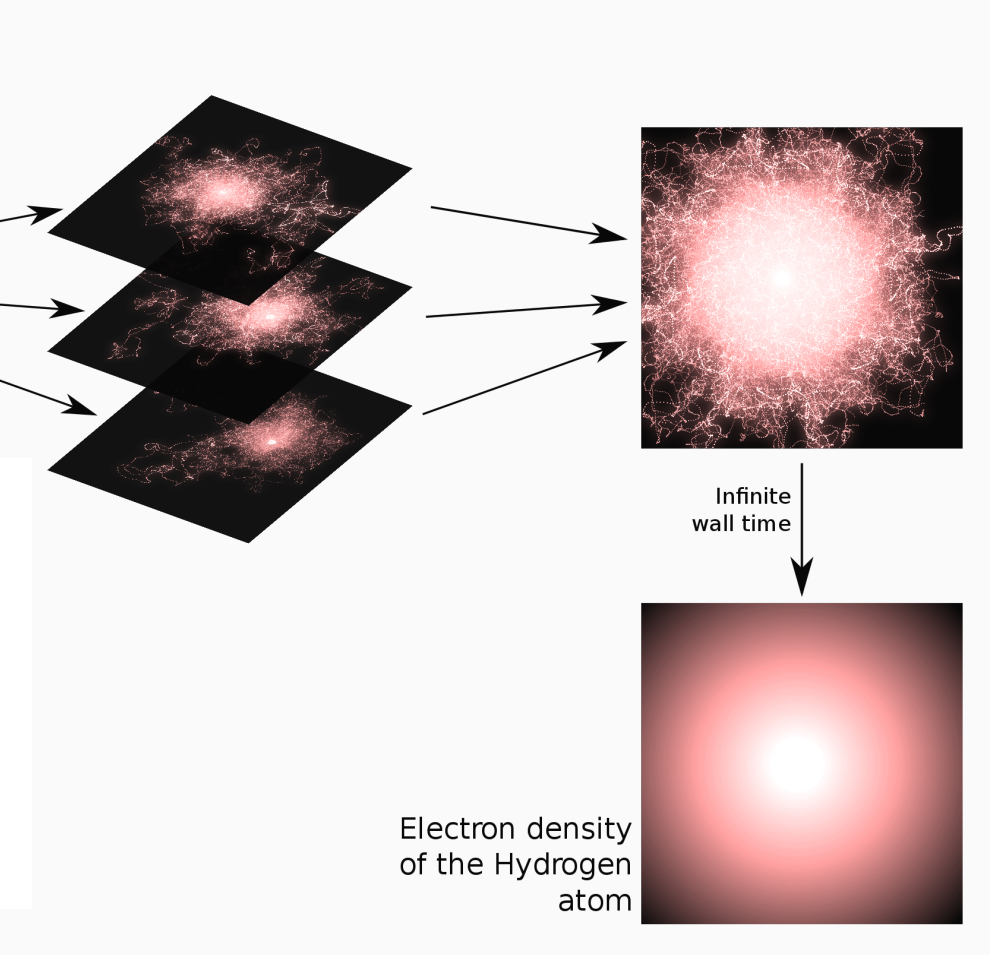
Here is an illustration of a trajectory:

Averaging all the trajectories converges to the density of the hydrogen atom.

The algorithm of the previous exercise is only slightly modified as:

Evaluate the local energy at $r_{n}$ and accumulate it
Compute a new position $r^{'} = r_{n} + δ t \frac{\nabla Ψ (r)}{Ψ (r)} + \sqrt{δ t} χ$
Evaluate $Ψ (r^{'})$ and $\frac{\nabla Ψ (r^{'})}{Ψ (r^{'})}$ at the new position
Compute the ratio $A = \frac{T (r^{'} \to r_{n}) P (r^{'})}{T (r_{n} \to r^{'}) P (r_{n})}$
Draw a uniform random number $v \in [0, 1]$
if $v \leq A$ , accept the move : set $r_{n + 1} = r^{'}$
else, reject the move : set $r_{n + 1} = r_{n}$

3.4.1. Gaussian random number generator

To obtain Gaussian-distributed random numbers, you can apply the Box Muller transform to uniform random numbers:

\begin{array}{rcl} z_{1} & = & \sqrt{- 2 \ln u_{1}} \cos (2 π u_{2}) \\ z_{2} & = & \sqrt{- 2 \ln u_{1}} \sin (2 π u_{2}) \end{array}

This gives Gaussian-distributed random numbers with zero mean and a variance of one.

Below is a Fortran and a C implementation returning a Gaussian-distributed n-dimensional vector $z$ . This will be useful for the following sections. In Python, you can use the random.normal function of Numpy.

If you use Fortran of C, copy/paste the random_gauss function in the qmc_stats.F90 or qmc_stats.c file.

Fortran

subroutine random_gauss(z,n)
  implicit none
  integer, intent(in) :: n
  double precision, intent(out) :: z(n)
  double precision :: u(n+1)
  double precision, parameter :: two_pi = 2.d0*dacos(-1.d0)
  integer :: i

  call random_number(u)

  if (iand(n,1) == 0) then
     ! n is even
     do i=1,n,2
        z(i)   = dsqrt(-2.d0*dlog(u(i))) 
        z(i+1) = z(i) * dsin( two_pi*u(i+1) )
        z(i)   = z(i) * dcos( two_pi*u(i+1) )
     end do

  else
     ! n is odd
     do i=1,n-1,2
        z(i)   = dsqrt(-2.d0*dlog(u(i))) 
        z(i+1) = z(i) * dsin( two_pi*u(i+1) )
        z(i)   = z(i) * dcos( two_pi*u(i+1) )
     end do

     z(n)   = dsqrt(-2.d0*dlog(u(n))) 
     z(n)   = z(n) * dcos( two_pi*u(n+1) )

  end if

end subroutine random_gauss

void random_gauss(double* z, size_t n);

#include <stdlib.h>
void random_gauss(double* z, size_t n) {
    double u[n+1];
    double two_pi = 2.0 * acos(-1.0);
    size_t i;

    //generate random numbers
    for (i = 0; i <= n; i++) {
        u[i] = drand48();
    }

    if (n % 2 == 0) {
        // n is even
        for (i = 0; i < n; i += 2) {
            z[i]   = sqrt(-2.0 * log(u[i]));
            z[i+1] = z[i] * sin(two_pi * u[i+1]);
            z[i]   = z[i] * cos(two_pi * u[i+1]);
        }
    } else {
        // n is odd
        for (i = 0; i < n-1; i += 2) {
            z[i]   = sqrt(-2.0 * log(u[i]));
            z[i+1] = z[i] * sin(two_pi * u[i+1]);
            z[i]   = z[i] * cos(two_pi * u[i+1]);
        }
        z[n-1] = sqrt(-2.0 * log(u[n-1]));
        z[n-1] = z[n-1] * cos(two_pi * u[n]);
    }
}

3.4.2. Exercise 1

Write a function to compute the drift vector $\frac{\nabla Ψ (r)}{Ψ (r)}$ .

Python
```
def drift(a,r):
   # TODO
```

Fortran

subroutine drift(a,r,b)
  implicit none
  double precision, intent(in)  :: a, r(3)
  double precision, intent(out) :: b(3)

  ! TODO

end subroutine drift

void drift(double a, double r[3], double b[3]) {
  //TODO
}

3.4.3. Exercise 2

Modify the previous program to introduce the drift-diffusion scheme. (This is a necessary step for the next section on diffusion Monte Carlo).

Python

#!/usr/bin/env python3

from hydrogen  import *
from qmc_stats import *

def MonteCarlo(a,nmax,dt):
   # TODO

# Run simulation
a    = 1.2
nmax = 100000
dt   = # TODO

X0 = [ MonteCarlo(a,nmax,dt) for i in range(30)]

# Energy
X = [ x for (x, _) in X0 ]
E, deltaE = ave_error(X)
print(f"E = {E} +/- {deltaE}")

# Acceptance rate
X = [ x for (_, x) in X0 ]
A, deltaA = ave_error(X)
print(f"A = {A} +/- {deltaA}")

Fortran

subroutine variational_montecarlo(a,nmax,dt,energy,accep)
  implicit none
  double precision, intent(in)  :: a, dt
  integer*8       , intent(in)  :: nmax 
  double precision, intent(out) :: energy, accep

  integer*8        :: istep
  integer*8        :: n_accep
  double precision :: sq_dt, chi(3)
  double precision :: psi_old, psi_new
  double precision :: r_old(3), r_new(3)
  double precision :: d_old(3), d_new(3)

  double precision, external :: e_loc, psi

  ! TODO

end subroutine variational_montecarlo

program qmc
  implicit none
  double precision, parameter :: a     = 1.2d0
  double precision, parameter :: dt    = ! TODO
  integer*8       , parameter :: nmax  = 100000
  integer         , parameter :: nruns = 30

  integer          :: irun
  double precision :: X(nruns), accep(nruns)
  double precision :: ave, err

  do irun=1,nruns
     call variational_montecarlo(a,nmax,dt,X(irun),accep(irun))
  enddo

  call ave_error(X,nruns,ave,err)
  print *, 'E = ', ave, '+/-', err

  call ave_error(accep,nruns,ave,err)
  print *, 'A = ', ave, '+/-', err

end program qmc

gfortran hydrogen.F90 qmc_stats.F90 vmc_metropolis.F90 -o vmc_metropolis
./vmc_metropolis

#include <stdio.h>
#include <stdlib.h>
#include <stddef.h> // for size_t
#include <math.h>
#include <time.h>
#include "hydrogen.h"
#include "qmc_stats.h"

void variational_montecarlo(double a, size_t nmax, double dt, 
                            double *energy, double *accep)
{
  // TODO
}


int main(void) {

#define a      1.2
#define nmax   100000
#define dt     // TODO
#define nruns  30

    double X[nruns];
    double Y[nruns];
    double ave, err;

    srand48(time(NULL));

    for (size_t irun = 0; irun < nruns; irun++) {
        variational_montecarlo(a, nmax, dt, &X[irun], &Y[irun]);
    }

    ave_error(X, nruns, &ave, &err);
    printf("E = %f +/- %f\n", ave, err);

    ave_error(Y, nruns, &ave, &err);
    printf("A = %f +/- %f\n", ave, err);

    return 0;
}

Contents:

4. Diffusion Monte Carlo

As we have seen, Variational Monte Carlo is a powerful method to compute integrals in large dimensions. It is often used in cases where the expression of the wave function is such that the integrals can't be evaluated (multi-centered Slater-type orbitals, correlation factors, etc).

Diffusion Monte Carlo is different. It goes beyond the computation of the integrals associated with an input wave function, and aims at finding a near-exact numerical solution to the Schrödinger equation.

4.1. Schrödinger equation in imaginary time

Consider the time-dependent Schrödinger equation:

$i \frac{\partial Ψ (r, t)}{\partial t} = (\hat{H} - E_{r e f}) Ψ (r, t) .$

where we introduced a shift in the energy, $E_{r e f}$ , for reasons which will become apparent below.

We can expand a given starting wave function, $Ψ (r, 0)$ , in the basis of the eigenstates of the time-independent Hamiltonian, $Φ_{k}$ , with energies $E_{k}$ :

$Ψ (r, 0) = \sum_{k} a_{k} Φ_{k} (r) .$

The solution of the Schrödinger equation at time $t$ is

$Ψ (r, t) = \sum_{k} a_{k} \exp (- i (E_{k} - E_{r e f}) t) Φ_{k} (r) .$

Now, if we replace the time variable $t$ by an imaginary time variable $τ = i t$ , we obtain

$- \frac{\partial ψ (r, τ)}{\partial τ} = (\hat{H} - E_{r e f}) ψ (r, τ)$

where $ψ (r, τ) = Ψ (r, - i τ)$ and

\begin{array}{rcl} ψ (r, τ) & = & \sum_{k} a_{k} \exp (- (E_{k} - E_{r e f}) τ) Φ_{k} (r) \\ = & \exp (- (E_{0} - E_{r e f}) τ) \sum_{k} a_{k} \exp (- (E_{k} - E_{0}) τ) Φ_{k} (r) . \end{array}

For large positive values of $τ$ , $ψ$ is dominated by the $k = 0$ term, namely, the lowest eigenstate. If we adjust $E_{r e f}$ to the running estimate of $E_{0}$ , we can expect that simulating the differential equation in imaginary time will converge to the exact ground state of the system.

4.2. Relation to diffusion

The diffusion equation of particles is given by

$\frac{\partial ψ (r, t)}{\partial t} = D Δ ψ (r, t)$

where $D$ is the diffusion coefficient. When the imaginary-time Schrödinger equation is written in terms of the kinetic energy and potential,

$\frac{\partial ψ (r, τ)}{\partial τ} = (\frac{1}{2} Δ - [V (r) - E_{r e f}]) ψ (r, τ),$

it can be identified as the combination of:

a diffusion equation (Laplacian)
an equation whose solution is an exponential (potential)

The diffusion equation can be simulated by a Brownian motion:

$r_{n + 1} = r_{n} + \sqrt{δ t} χ$

where $χ$ is a Gaussian random variable, and the potential term can be simulated by creating or destroying particles over time (a so-called branching process) or by simply considering it as a cumulative multiplicative weight along the diffusion trajectory (pure Diffusion Monte Carlo):

$\prod_{i} \exp (- (V (r_{i}) - E_{ref}) δ t) .$

We note that the ground-state wave function of a Fermionic system is antisymmetric and changes sign. Therefore, its interpretation as a probability distribution is somewhat problematic. In fact, mathematically, since the Bosonic ground state is lower in energy than the Fermionic one, for large $τ$ , the system will evolve towards the Bosonic solution.

For the systems you will study, this is not an issue:

Hydrogen atom: You only have one electron!
Two-electron system ( $H_{2}$ or He): The ground-wave function is antisymmetric in the spin variables but symmetric in the space ones.

Therefore, in both cases, you are dealing with a "Bosonic" ground state.

4.3. Importance sampling

In a molecular system, the potential is far from being constant and, in fact, diverges at the inter-particle coalescence points. Hence, it results in very large fluctuations of the weight associated with the potential, making the calculations impossible in practice. Fortunately, if we multiply the Schrödinger equation by a chosen trial wave function $Ψ_{T} (r)$ (Hartree-Fock, Kohn-Sham determinant, CI wave function, etc), one obtains

$- \frac{\partial ψ (r, τ)}{\partial τ} Ψ_{T} (r) = [- \frac{1}{2} Δ ψ (r, τ) + V (r) ψ (r, τ)] Ψ_{T} (r)$

Defining $Π (r, τ) = ψ (r, τ) Ψ_{T} (r)$ , (see appendix for details)

$- \frac{\partial Π (r, τ)}{\partial τ} = - \frac{1}{2} Δ Π (r, τ) + \nabla [Π (r, τ) \frac{\nabla Ψ_{T} (r)}{Ψ_{T} (r)}] + (E_{L} (r) - E_{r e f}) Π (r, τ)$

The new "kinetic energy" can be simulated by the drift-diffusion scheme presented in the previous section (VMC). The new "potential" is the local energy, which has smaller fluctuations when $Ψ_{T}$ gets closer to the exact wave function. This term can be simulated by $\prod_{i} \exp (- (E_{L} (r_{i}) - E_{ref}) δ t) .$ where $E_{r e f}$ is the constant we had introduced above, which is adjusted to an estimate of the average energy to keep the weights close to one.

This equation generates the N-electron density $Π$ , which is the product of the ground state solution with the trial wave function. You may then ask: how can we compute the total energy of the system?

To this aim, we use the mixed estimator of the energy:

\begin{array}{rcl} E (τ) & = & \frac{⟨ ψ (τ) | \hat{H} | Ψ_{T} ⟩}{⟨ ψ (τ) | Ψ_{T} ⟩} \\ = & \frac{\int ψ (r, τ) \hat{H} Ψ_{T} (r) d r}{\int ψ (r, τ) Ψ_{T} (r) d r} \\ = & \frac{\int ψ (r, τ) Ψ_{T} (r) E_{L} (r) d r}{\int ψ (r, τ) Ψ_{T} (r) d r} . \end{array}

For large $τ$ , we have that

$Π (r, τ) = ψ (r, τ) Ψ_{T} (r) \to Φ_{0} (r) Ψ_{T} (r),$

and, using that $\hat{H}$ is Hermitian and that $Φ_{0}$ is an eigenstate of the Hamiltonian, we obtain for large $τ$

$E (τ) = \frac{⟨ ψ_{τ} | \hat{H} | Ψ_{T} ⟩}{⟨ ψ_{τ} | Ψ_{T} ⟩} = \frac{⟨ Ψ_{T} | \hat{H} | ψ_{τ} ⟩}{⟨ Ψ_{T} | ψ_{τ} ⟩} \to E_{0} \frac{⟨ Ψ_{T} | Φ_{0} ⟩}{⟨ Ψ_{T} | Φ_{0} ⟩} = E_{0}$

Therefore, we can compute the energy within DMC by generating the density $Π$ with random walks, and simply averaging the local energies computed with the trial wave function.

4.3.1. Appendix : Details of the Derivation

$- \frac{\partial ψ (r, τ)}{\partial τ} Ψ_{T} (r) = [- \frac{1}{2} Δ ψ (r, τ) + V (r) ψ (r, τ)] Ψ_{T} (r)$

$- \frac{\partial [ψ (r, τ) Ψ_{T} (r)]}{\partial τ} = - \frac{1}{2} (Δ [ψ (r, τ) Ψ_{T} (r)] - ψ (r, τ) Δ Ψ_{T} (r) - 2 \nabla ψ (r, τ) \nabla Ψ_{T} (r)) + V (r) ψ (r, τ) Ψ_{T} (r)$

$- \frac{\partial [ψ (r, τ) Ψ_{T} (r)]}{\partial τ} = - \frac{1}{2} Δ [ψ (r, τ) Ψ_{T} (r)] + \frac{1}{2} ψ (r, τ) Δ Ψ_{T} (r) + Ψ_{T} (r) \nabla ψ (r, τ) \frac{\nabla Ψ_{T} (r)}{Ψ_{T} (r)} + V (r) ψ (r, τ) Ψ_{T} (r)$

$- \frac{\partial [ψ (r, τ) Ψ_{T} (r)]}{\partial τ} = - \frac{1}{2} Δ [ψ (r, τ) Ψ_{T} (r)] + ψ (r, τ) Δ Ψ_{T} (r) + Ψ_{T} (r) \nabla ψ (r, τ) \frac{\nabla Ψ_{T} (r)}{Ψ_{T} (r)} + E_{L} (r) ψ (r, τ) Ψ_{T} (r)$ $- \frac{\partial [ψ (r, τ) Ψ_{T} (r)]}{\partial τ} = - \frac{1}{2} Δ [ψ (r, τ) Ψ_{T} (r)] + \nabla [ψ (r, τ) Ψ_{T} (r) \frac{\nabla Ψ_{T} (r)}{Ψ_{T} (r)}] + E_{L} (r) ψ (r, τ) Ψ_{T} (r)$

Defining $Π (r, t) = ψ (r, τ) Ψ_{T} (r)$ ,

$- \frac{\partial Π (r, τ)}{\partial τ} = - \frac{1}{2} Δ Π (r, τ) + \nabla [Π (r, τ) \frac{\nabla Ψ_{T} (r)}{Ψ_{T} (r)}] + E_{L} (r) Π (r, τ)$

Contents:

4.3.1. Appendix : Details of the Derivation

4.4. Pure Diffusion Monte Carlo

Instead of having a variable number of particles to simulate the branching process as in the Diffusion Monte Carlo (DMC) algorithm, we use variant called pure Diffusion Monte Carlo (PDMC) where the potential term is considered as a cumulative product of weights:

\begin{array}{r} W (r_{n}, τ) = \prod_{i = 1}^{n} \exp (- δ t (E_{L} (r_{i}) - E_{ref})) = \prod_{i = 1}^{n} w (r_{i}) \end{array}

where $r_{i}$ are the coordinates along the trajectory and we introduced a time-step variable $δ t$ to discretize the integral.

The PDMC algorithm is less stable than the DMC algorithm: it requires to have a value of $E_{ref}$ which is close to the fixed-node energy, and a good trial wave function. Moreover, we can't let $τ$ become too large because the weight whether explode or vanish: we need to have a fixed value of $τ$ (projection time). The big advantage of PDMC is that it is rather simple to implement starting from a VMC code:

Start with $W (r_{0}) = 1, τ_{0} = 0$
Evaluate the local energy at $r_{n}$
Compute the contribution to the weight $w (r_{n}) = \exp (- δ t (E_{L} (r_{n}) - E_{ref}))$
Update $W (r_{n}) = W (r_{n - 1}) \times w (r_{n})$
Accumulate the weighted energy $W (r_{n}) \times E_{L} (r_{n})$ , and the weight $W (r_{n})$ for the normalization
Update $τ_{n} = τ_{n - 1} + δ t$
If $τ_{n} > τ_{max}$ ( $τ_{max}$ is an input parameter), the long projection time has been reached and we can start an new trajectory from the current position: reset $W (r_{n}) = 1$ and $τ_{n} = 0$
Compute a new position $r^{'} = r_{n} + δ t \frac{\nabla Ψ (r)}{Ψ (r)} + \sqrt{δ t} χ$
Evaluate $Ψ (r^{'})$ and $\frac{\nabla Ψ (r^{'})}{Ψ (r^{'})}$ at the new position
Compute the ratio $A = \frac{T (r^{'} \to r_{n}) P (r^{'})}{T (r_{n} \to r^{'}) P (r_{n})}$

Draw a uniform random number $v \in [0, 1]$
if $v \leq A$ , accept the move : set $r_{n + 1} = r^{'}$
else, reject the move : set $r_{n + 1} = r_{n}$

Some comments are needed:

You estimate the energy as
$\begin{array}{r} E = \frac{\sum_{k = 1}^{N_{M C}} E_{L} (r_{k}) W (r_{k}, k δ t)}{\sum_{k = 1}^{N_{M C}} W (r_{k}, k δ t)} \end{array}$
The result will be affected by a time-step error (the finite size of $δ t$ ) due to the discretization of the integral, and one has in principle to extrapolate to the limit $δ t \to 0$ . This amounts to fitting the energy computed for multiple values of $δ t$ .

Here, you will be using a small enough time-step and you should not worry about the extrapolation.
The accept/reject step (steps 9-12 in the algorithm) is in principle not needed for the correctness of the DMC algorithm. However, its use reduces significantly the time-step error.

4.5. Hydrogen atom

4.5.1. Exercise

Modify the Metropolis VMC program into a PDMC program. In the limit $δ t \to 0$ , you should recover the exact energy of H for any value of $a$ , as long as the simulation is stable. We choose here a time step of 0.05 a.u. and a fixed projection time $τ_{max}$ =100 a.u.

Python

from hydrogen  import *
from qmc_stats import *

def MonteCarlo(a, nmax, dt, Eref):
    # TODO

# Run simulation
a     = 1.2
nmax  = 100000
dt    = 0.05
tau   = 100.
E_ref = -0.5

X0 = [ MonteCarlo(a, nmax, dt, E_ref) for i in range(30)]

# Energy
X = [ x for (x, _) in X0 ]
E, deltaE = ave_error(X)
print(f"E = {E} +/- {deltaE}")

# Acceptance rate
X = [ x for (_, x) in X0 ]
A, deltaA = ave_error(X)
print(f"A = {A} +/- {deltaA}")

Fortran

subroutine pdmc(a, nmax, dt, energy, accep, tau, E_ref)
  implicit none
  double precision, intent(in)  :: a, dt, tau
  integer*8       , intent(in)  :: nmax 
  double precision, intent(out) :: energy, accep
  double precision, intent(in)  :: E_ref

  integer*8        :: istep
  integer*8        :: n_accep
  double precision :: sq_dt, chi(3)
  double precision :: psi_old, psi_new
  double precision :: r_old(3), r_new(3)
  double precision :: d_old(3), d_new(3)

  double precision, external :: e_loc, psi

  ! TODO

end subroutine pdmc

program qmc
  implicit none
  double precision, parameter :: a     = 1.2d0
  double precision, parameter :: dt    = 0.05d0
  double precision, parameter :: E_ref = -0.5d0
  double precision, parameter :: tau   = 100.d0
  integer*8       , parameter :: nmax  = 100000
  integer         , parameter :: nruns = 30

  integer          :: irun
  double precision :: X(nruns), accep(nruns)
  double precision :: ave, err

  do irun=1,nruns
     call pdmc(a, nmax, dt, X(irun), accep(irun), tau, E_ref)
  enddo

  call ave_error(X,nruns,ave,err)
  print *, 'E = ', ave, '+/-', err

  call ave_error(accep,nruns,ave,err)
  print *, 'A = ', ave, '+/-', err

end program qmc

gfortran hydrogen.F90 qmc_stats.F90 pdmc.F90 -o pdmc
./pdmc

#include <stdio.h>
#include <stdlib.h>
#include <stddef.h> // for size_t
#include <math.h>
#include <time.h>
#include "hydrogen.h"
#include "qmc_stats.h"

void pdmc(double a, size_t nmax, double dt, double *energy, double *accep,
          double tau, double e_ref)
{
  // TODO
}


int main(void) {

#define a      1.2
#define nmax   100000
#define dt     0.05
#define tau    100.0
#define e_ref  -0.5
#define nruns  30

    double X[nruns];
    double Y[nruns];
    double ave, err;

    srand48(time(NULL));

    for (size_t irun = 0; irun < nruns; irun++) {
        pdmc(a, nmax, dt, &X[irun], &Y[irun], tau, e_ref);
    }

    ave_error(X, nruns, &ave, &err);
    printf("E = %f +/- %f\n", ave, err);

    ave_error(Y, nruns, &ave, &err);
    printf("A = %f +/- %f\n", ave, err);

    return 0;
}

gcc hydrogen.c qmc_stats.c pdmc.c -lm -o pdmc
./pdmc

Contents:

4.5.1. Exercise

Contents:

5. Project

Change your PDMC code for one of the following:

the Helium atom, or
the H₂ molecule at $R$ =1.401 bohr.

And compute the ground state energy.

Top: Quantum Monte CarloHELP / toggle view
Previous \| Next	Table of Contents	1

Quantum Monte Carlo

Quantum Monte Carlo

Table of Contents

Quantum Monte Carlo

Table of Contents

1. Introduction

1.1. Energy and local energy

2. Numerical evaluation of the energy of the hydrogen atom

2.1. Local energy

2.1.1. Test-driven development

2.1.2. Exercise 1

2.1.3. Exercise 2

2.1.4. Exercise 3

2.1.5. Exercise 4

2.1.6. Exercise 5

2.2. Plot of the local energy along the x axis

2.2.1. Exercise

2.3. Numerical estimation of the energy

2.3.1. Exercise

2.4. Variance of the local energy

2.4.1. Exercise (optional)

2.4.2. Exercise

3. Variational Monte Carlo

3.1. Computation of the statistical error

3.1.1. Exercise

3.2. Uniform sampling in the box

3.2.1. Exercise

3.3. Metropolis sampling with Ψ2

3.3.1. Optimal step size

3.3.2. Exercise

3.4. Generalized Metropolis algorithm

3.4.1. Gaussian random number generator

3.4.2. Exercise 1

3.4.3. Exercise 2

4. Diffusion Monte Carlo

4.1. Schrödinger equation in imaginary time

4.2. Relation to diffusion

4.3. Importance sampling

4.3.1. Appendix : Details of the Derivation

4.4. Pure Diffusion Monte Carlo

4.5. Hydrogen atom

4.5.1. Exercise

5. Project

6. Acknowledgments

2.2. Plot of the local energy along the $x$ axis

3.3. Metropolis sampling with Ψ²