Transcorrelated calculations
HOME
Table of Contents
Congratulations! By reaching this point in the tutorial, you have made fantastic progress and are one step closer to mastering the QP code. In this part of the tutorial you will learn how you can easily run a calculation with an explicitly correlated wavefunction in the framework of the Transcorrelated (TC) theory.
1 CI vs CI-Jastrow wavefunction
In the precious sections, all the ground and the excited states calculations were made with a CI wavefunction, \[ \Psi = \sum_I c_I D_I \] where \(D_I\) are the Slater determinants. In this section, we will go one step further to include dynamical correlation via a Jastrow factor, \[ \Psi = \sum_I c_I D_I e^{\tau}. \] The Jastrow factor implemented in the QP has the following expression, \[ \tau = \sum_{i,j} u(r_{ij}) v(r_i) v(r_j), \] where the 2-electron function is inspired by range-separated DFT, \[ u(r_{12}) = \frac{r_{12} \, \left[ 1 - \text{erf} \left( \mu r_{12} \right) \right]}{2} - \frac{\exp \left[ -\left( \mu r_{12} \right)^2 \right] }{2 \sqrt{\pi} \mu} \] and \(v\) is an envelope that has been added to cancel out the correlation when electrons are closed to nuclei, \[ v(\mathbf{r}) = \Pi_A \left[ 1 - \exp \left( -\alpha_A \left( \mathbf{r} - \mathbf{R_A} \right)^2 \right) \right], \] where the index \(A\) runs over the nuclei. The parameter \(\mu\) controls both the depth of the coulomb hole and the typical range of the correlation factor in \(r_{12}\). In practice, \(\mu=0.87\) is optimal to correlate valence electrons and therefore only the parameter \(\alpha\) need to be optimized. This parameter depends on the atom as well as the choice of the basis set. In this tutorial, the optimal value of \(\alpha\) will be given.
2 Installation
Since the TC algorithms are developed very recently, you need to
switch from master to dev-stable-tc-scf. This can be done easily
by few steps.
First go to the repository of QP and then switch to the branch of TC development
cd qp2
git checkout -b dev-stable-tc-scf
Pull the TC codes to your repository by doing
git pull origin dev-stable-tc-scf
Now compile the code by doing
ninja clean
ninja
Make sure that you have sourced before compiling
source quantum_package.rc
Now you can start running TC calculation! ;)
3 TC self consistent field
In the standard post-Hartree-Fock methods, the Hartree-Fock (HF) orbitals provide a good start point. Although we can use the HF orbitals in the TC calculations, it is better to start from optimized orbitals to accelerate the convergence in term of the number of determinants. The TC self consistent field TC-SCF is an iterative method that allows to get canonical biorthogonal left \(\{\chi_i\}\) and right \(\{\phi_i\}\) orbitals, \[ \left\langle \chi_i | \phi_j \right\rangle = \delta_{ij} \] that make the TC energy stationary at the one-determinantal level. These orbitals satisfies the Brillouin theorem for the TC Hamiltonian.
In order to show how to run a TC-SCF calculation, we consider again the example
of the dinitrogen with the cc-pVDZ basis set, at a distance of 2.118 atomic units.
We start by creating an EZFIO database and running a standard HF calculation that
will be used as a start point for the TC-SCF.
Don't forget to create the z-matrix file n2.zmt before creating the EZFIO.
qp create_ezfio --au -b cc-pvdz n2.zmt -o n2_tc
qp run scf | tee n2_tc.scf.out
Before performing the TC-SCF calculation we need to fix the parameters
of the Jastrow.
Many Jastrow factor are under development in QP. The form discussed above
corresponds to the keyword j1b_type=3
qp set tc_keywords j1b_type 3
Concerning the parameter \(\mu\) of the Jastrow, it is recommended to use always \(\mu=0.87\).
qp set ao_two_e_erf_ints mu_erf 0.87
The parameter \(\alpha\) need to be optimized in general for each atom and the optimal value depends on the basis sets. For the Nitrogen atom in cc-pVDZ, the optimal correlation parameter is \(\alpha=1.4\).
qp set tc_keywords j1b_pen "[1.4, 1.4]"
Since TC integrals can be expensive to calculate, once they are calculated, we store them in the EZFIO database. This allows them to be read directly in a future calculation (like in the next TC-CIPSI calculation). This can be done with,
qp set tc_keywords io_tc_integ Write
We can now run the tc-scf code and save the output in a file
n2_tc.tc_scf.out by doing
qp run tc_scf |tee n2_tc.tc_scf.out
To check the obtained energy by searching TC energy = in the
output file, or by the command
qp get tc_scf bitc_energy
The expected TC-SCF energy is -109.001278 atomic units. In contrast to the HF energy which, by definition, does not include electronic correlation, the TC-SCF energy includes correlation although only one determinant is used. This is why we get an improvement with respect to the HF energy by \(\approx 52\) mH.
4 TC CIPSI
In the previous sections, we observed that CIPSI is highly
efficient in approximating the FCI energy. In this section, we
will delve into the accuracy of TC-CIPSI and demonstrate how
it achieves near TC-FCI accuracy.
Additionally, we will compare the results obtained from CIPSI
and TC-CIPSI, shedding light on the similarities and differences
between the two methods. To ensure a fair comparison, we will
freeze the core orbitals and maintain the same number of of
n_det_max as before:
qp set_frozen_core
qp set determinants n_det_max 50000
We proceed now to the TC-CIPSI calculation via the fci_tc_bi_ortho
code and we save the output to the file n2_tc.tcfci.out:
qp run fci_tc_bi_ortho |tee n2_tc.tcfci.out
The output file contains a lot of information.
To extract the relevant data and visualize the convergence of the
TC energy in function of the number of determinants, we can
simply use the grep command:
grep "Ndet,E,E+PT2,E+RPT2,|PT2|=" n2_tc.tcfci.out | cut -d "=" -f 2 > data_tc
data_tc contains 5 columns.
These columns refer to the number of selected determinants
N_det, the TC energy in the basis of selected determinants \(E_{TC}^{0}\),
the estimation of the TC-FCI energy with the TC-PT2 correction
\(E_{TC}^{0}+E_{TC}^{2}\) and with renormalized correction TC-rPT2
\(E_{TC}^{0}+rE_{TC}^{2}\), and finally the negative part of the TC-PT2 correction.
Note that in the standard case the PT2 is always negative while the TC-PT2
may be positive or negative depending on the chosen Jastrow factor.
4.1 Convergence of TC-CIPSI
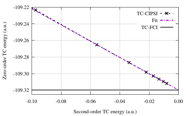
First we want to compare between the obtained TC-CIPSI energy and the TC-FCI energy \(E_{\text{TC-FCI}}=-109.3199\) atomic units.
The extrapolation of the TC-CIPSI energy \[ E_{\text{TC-CIPSI}}^{0}(E_{\text{TC-CIPSI}}^{2}) \approx a (E_{\text{TC-CIPSI}}^{2}) + E_{\text{TC-FCI}} \] gives an estimation of \(E_{\text{TC-FCI}} \approx -109.3197\) atomic units which is very close to the TC-FCI energy.
#!/usr/bin/gnuplot
set terminal pdfcairo enhanced font "Times,12"  size 4.0,2.5
set output "extrap_Etc.pdf"

set grid

set format x "%.2f"
set xrange [-0.10:0]
set xlabel "Second-order TC energy (a.u.)"

set yrange[-109.325:*]
set ylabel "Zero-order TC energy (a.u.)"
set format y "%.2f"

E_TCCIPSI(E_TCPT2) = a * E_TCPT2 + E_TCFCI
fit [-0.05:0.] E_TCCIPSI(x) "data_tc" using ($4-$2):2 via a, E_TCFCI
print E_TCFCI

plot "data_tc" u ($4-$2):2 t "TC-CIPSI" w lp lt 2 dt 2 lw 2.0 lc 0 pt 2 ps 0.7 \
  , E_TCCIPSI(x)           t "Fit"      w l  lt 4 dt 4 lw 2.0 lc 1             \
  , -109.3199              t "TC-FCI"   w l  lt 1 dt 1 lc 0 lw 2.0             \

set encoding iso_8859_1
exit

4.2 CIPSI vs TC-CIPSI
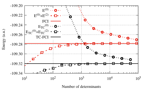
We turn now to the comparison between the CIPSI and the TC-CIPSI energies. The following gnuplot script allows to visualize the convergence of both, in term of the number of determinants.
#!/usr/bin/gnuplot
set terminal pdfcairo enhanced font "Times,12"  size 4.0,2.5
set output "conv_Etc.pdf"

set grid
#set key top right

set xrange [10:100000]
set logscale x
set xlabel "Number of determinants"
set format x "10^{%L}"

set yrange [-109.34:-109.20]
set ylabel "Energy (a.u.)"
set format y "%.2f"

set key top left

plot "data"    u 1:2        t "E^{(0)}"                   w lp lt 3 dt 3 lc 7 lw 3.0 pt 6 ps 0.7 \
   , "data"    u 1:($2+$3)  t "E^{(0)}+E^{(2)}"           w lp lt 2 dt 2 lc 7 lw 2.0 pt 4 ps 0.7 \
   , -109.278339            t "FCI"                       w l  lt 1 dt 1 lc 7 lw 2.0             \
   , "data_tc" u 1:2        t "E_{TC}^{(0)}"              w lp lt 3 dt 3 lc 0 lw 3.0 pt 6 ps 0.7 \
   , "data_tc" u 1:3        t "E_{TC}^{(0)}+E_{TC}^{(2)}" w lp lt 2 dt 2 lc 0 lw 2.0 pt 4 ps 0.7 \
   , -109.3199              t "TC-FCI"                    w l  lt 1 dt 1 lc 0 lw 2.0             \

set encoding iso_8859_1
exit

We observe that both \(E_{\text{CISPI}}\) and \(E_{\text{TC-CISPI}}\) converge to the \(E_{\text{FCI}}\) and \(E_{\text{TC-FCI}}\) limits, respectively. However, the TC energy provide an improvement over the standard FCI energy by \(\approx 41\) mH.